UChicago Trading Competition 2024: A Reflection on the Market Making Intuition
April 20th 2024
Last weekend, I had the pleasure to make a trip to the University of Chicago to participate in their annual trading competition. Even though the competition itself spans less than a day, preparations for it silently took place throughout the week leading up to the competition day. Teams were tasked with developing a trading strategy that would maximize the expected PnL of a small portfolio of assets, with only 5 stocks, 2 exchange-traded funds (ETFs), and a risk-free asset.Normally, it would make more sense for the winners to do a writeup of their strategies. But as our team dominated the leaderboards during the run-up to and even the early phase of the competition, yet ended up in the middle of the pack, I thought it would also be interesting to share my experience and reflections on the competition. Additionally, I want to discuss (albeit scratching the surface), several winning approaches that have been employed by the top teams, and how we can improve upon them in the future.
The Case
Your fantasy hedge fund has been given a portfolio of 5 stocks (EPT, DLO, MKU, IGM, BRV), 2 ETFs (SCP, JAK), and a risk-free asset (JMS). For each stock, we have the option to either place a market order or a limit order. The market order is executed at the best available price, while the limit order is executed at a specified price or better. An ETF can be thought of as an agreement between parties on the exchange; one can swap (for a small fee!) between 10 shares of JCR and 3 EPT, 3 IGM, 4 BRV. The forward direction is known as a redemption, and the backward as creation.- Creation: You give 3 EPT, 3 IGM, 4 BRV to the ETF provider. You get 10 shares of the ETF from the provider.
- Redemption: You return 10 shares of JCR to the ETF provider. You then receive 3 EPT, 3 IGM, and 4 BDR from the provider.
Therefore, we decided to focus on the market making aspect of the competition, and take advantage of the spread between the bid and ask prices. But then, we were faced with the problem of other naive bots and desperate buyers/sellers who would scramble for even the most unreasonable prices. How can we produce a reasonable prediction based on the given data, as well as live market conditions?
Strategies
(Naive) Strategy 1: Buy Low, Sell High
When we carried out the EDA for this case, it is not difficult to notice that the settlement prices are relatively normally distributed. For example, this is the histogram of the settlement prices of EPT, where the distribution is estimated using Kernel Density Estimation (KDE).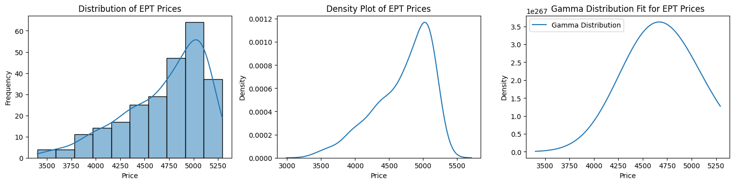 This means that we can hard-code a median value, where we would buy if the price is below the median (i.e. there is more than 50% chance that the price will go up), and
sell otherwise. This strategy is simple and intuitive, and indeed sounds almost too good to be true in a volatile market, where the price can swing wildly in a matter of seconds.
Yet, in a more informed market, this strategy proves to be disastrous, as we will likely be betting against rising stocks, and holding falling assets.
This means that we can hard-code a median value, where we would buy if the price is below the median (i.e. there is more than 50% chance that the price will go up), and
sell otherwise. This strategy is simple and intuitive, and indeed sounds almost too good to be true in a volatile market, where the price can swing wildly in a matter of seconds.
Yet, in a more informed market, this strategy proves to be disastrous, as we will likely be betting against rising stocks, and holding falling assets.
(Naive) Strategy 2: Penny In-Penny Out (PIPO)
The idea behind this strategy is to make a small profit on each trade, while maximizing the number of completed orders. We achieve this by placing a limit order at one cent above the highest bid, and one cent below the lowest ask. This strategy is particularly useful in a market where the spread is large, and the price is relatively stable. However, in a volatile market, this strategy is not only unprofitable, but also risky, as we would be trading more frequently, and thus incurring more transaction costs.What has been surprising to us is the frequency that the PIPO strategy appears in previous writeups, both for the UChicago Trading Competition and other similar events. Some resources are listed in the References below. It occurs to us from the very beginning that it is very difficult to make a cut in the competition if everyone is dependent on this strategy. Nonetheless, the strategy is still worth mentioning, as it is a good starting point for beginners to understand the market making process.
Strategy 3: ETF Arbitrage
One of the strategies that we have considered and implemented is the ETF Arbitrage strategy. The idea is to take advantage of the spread between the predicted price of the ETF and the actual price. For example, if 10 JAK is currently being traded at $100, but it only takes us $90 to buy the underlying stocks and $5 to create an ETF, then we can bag a profit of $5 by buying the stocks and creating an ETF. Nonetheless, it is apparent that this strategy heavily relies on a good prediction of the market prices, which we will present an extensive study of in the following section.After the competition, we found out that the ETF Arbitrage strategy has been key to the performance of some of this years highest-ranking teams. Of course, these teams have also implemented good predictions of the price series, which we will discuss in the next section. It is also noteworthy that the ETF Arbitrage strategy also requires a good observation of the current market volume. If the ETF cannot be sold after creation, and the market adjusts itself to the "correct" price, then we just lost $5 of conversion fee for nothing.
Strategy 4: Placing Level Orders
During the running-up to the competition, we noticed that there are many aggressive buyers and sellers who would place market orders at unreasonable prices. In order to take advantage of this, we decided to place limit orders at extreme prices, in a incrementing ladder to catch these orders. For example, if the current bid price is $100, we would place limit orders at $99.80, $99.60, $99.40, and so on, same for ask prices.This strategy seems to be the key to our dominance on the leaderboards during the run-up to the competition, when the market is relatively immature. Since our bots makes very fast and rapid decisions, we were able to catch the market orders of other bots, and constantly brings in at least $500 per round, very large compared to competition day average. However, as the market matures, and the bots become more sophisticated, this strategy becomes less useful, and even prone to punishments by hitters when the price swings in the opposite direction.
Strategy 5: Pair Tradings
As the given data was not in chronological order, we soon gave up hope on calculating the correlation and cointegration between the prices of the assets. Nonetheless, one of the team from UChicago did implement a pair trading strategy, and it seems to paid off, as the team finished third in case 1. The idea is to find two assets that are highly correlated, and place a long position on one and a short position on the other. I don't want to delve too much into this strategy, as I am not familiar with it, but I will leave you with the correlation matrix for your own contemplation: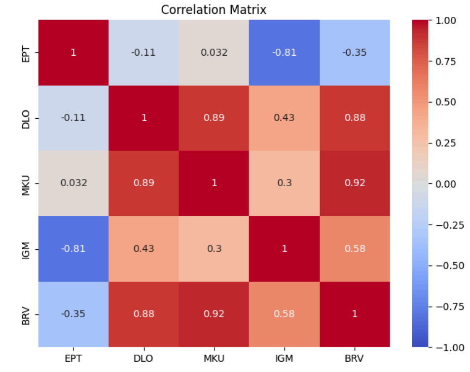
Predicting the fair price
One of the key aspects of the competition is to predict the fair price of the assets. This is particularly important in the ETF Arbitrage strategy, where we need to predict the price of the ETF in order to make a profit. We have tried several methods to predict the fair price, including:- Using Last Transacted Price
- Exponential Moving Average (EMA)
- Sliding Window Median
- Potential Energy Estimation
Using Last Transacted Price
This is the simplest method to predict the fair price. We simply take the last transacted price as the fair price. We improved upon a previous implementation of EnriqueKhai by separating the prediction of the fair price for bids and asks. This provides a very fast and relatively accurate estimation of the fair price in a stable market, allowing us to make high frequency trades and brings in constant profits. Despite having implemented multiple other complex predictors, we switched gear and opted for this prediction strategy barely one day before the competition (I even arrived in Chicago!). Nonetheless, this strategy is the least robust of all, as it is very sensitive to price swings and wrong predictions.To illustrate, let's consider the following simple example: the current fair price of EPT is at $40, and the last fulfilled bid is at $38 (for some reason, we made a huge profit there). But now, we are inclined to place bids at around $38, none of which are fulfilled, so our prediction of the fair bids fluctuates around $38. In a flourishing market, we end up selling a lot, eventually ended up stalling the negative limit of -200 EPT at $42. But the price keeps going up! At the end of the round, the price is at $46, and we have made a loss of $800.
In retrospect, this price prediction strategy is probably what decimated our performance in the competition. We barely noticed the discrepancy 45 minutes into the rounds, by then we have been trailing by a large margin.
Exponential Moving Average
The Exponential Moving Average (EMA) is a more sophisticated method to predict the fair price. It is a weighted average of the last n prices, where the weights decrease exponentially as we go back in time. Its formula is given by: $$\text{EMA} = (1-\alpha)\text{EMA} + \alpha \times P_n$$ where \(\alpha \) is chosen to be \(0.2\), and \(P_n\) is the observed price on day \(n\) of the round. A closer inspection of the formula shows a factor of \((1-\alpha)^i\) for a price observed \(i\) days ago, which does achieve the desired effect of decreasing the weight of older prices. One good thing about the EMA is that it is less sensitive to price swings, and thus provides a more stable prediction of the fair price. However, when the spread is tiny and the desired accuracy is high, the EMA is not as useful.Sliding Window Median
A common question raised in both the Case Packet and vehemently debated among teams is how do we differentiate between an informed and uninformed trader in a market where there are many uninformed traders who could easily trip us off with false prices? And who should we bet our predicted prices on?The Sliding Window Median addresses exactly that problem, by looking at the current order books, places heavy weights on order of large volumes, and calculate a reasonable middlepoint of the bid and ask. We essentially assume that if there is a large volume of orders at a certain price, then the bidder (asker) is likely to possess some information about the market that we don't, and thus the fair price is likely to be around that highly weighted price. The algorithm can be formulated as follows:
- Sort the prices in the order book in ascending order, disregard of bids or asks (some uninformed traders' ask can be lower than an informed trader's bid)
- Initialize a string \(s\)
- For each bid of volume \(v\), add \(v\) open parentheses to \(s\). For each ask of volume \(v\) add \(v\) closing parentheses to \(s\)
- Find the index \(i\) to minimize $$\mid O[i] - C[i] \mid$$ where \(O[i]\) is the number of opening parentheses to the left of \(i\), and \(C[i]\) is the number of closing parentheses to the right of \(i\)
- Then this index is closest to the fair price
In retrospect, having swapped out the Sliding Window Median is our (or at least mine) biggest regret of the competition, especially when the organizers have explicitly mentioned the increasing difficulty of hitters during the competition. During the training period, the SWM has constantly bring in about $30,000 per round. This was relatively small compared to some other teams whose range of PnL is in the hundreds of thousands, prompting us to switch to a faster and more aggressive approach.
Potential Energy Estimation
This method is actually my favorite of all, albeit its underdevelopment. The idea is to treat the original price distribution as a potential energy field, where the price is the height of the field, and calculate the gradient of the field to find the direction of the price movement. The algorithm can be formulated as follows: $$\delta(y|x,k) = f(x) - f(y) + \mu_k \int_x^y\left[\cos(\tan^{-1}(\frac{df}{dx}))\sqrt{1+f^2}\right]dx$$ where \(f\) is the PDF derived from the price distribution, \(k\) is the look-ahead window, and \(V\) is the variance of the PDF. The integral term can be thought of as the friction, which varies inverse-proportionally to \(V, k\). Solving for the equation above essentially gives us the destination with the smallest possible energy cost, and thus the most likely price movement.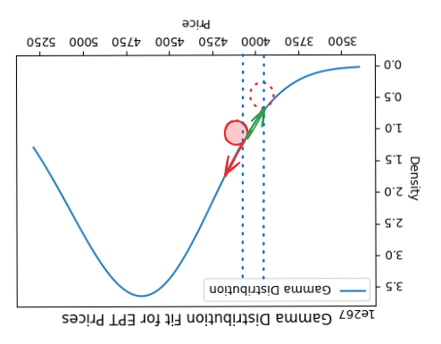
Now if you are a quick-witted mathematician, then you probably notice that the solution to this equation does not quite depend on \(\mu_k\) (which does not serve our purpose quite well). Post competition, my teammate Divyansh Shivashok actually came up with a slight modification of the model, which employs some particle-scale physics. But by this time we are just having fun with this predictor, and it might worth dwelling into in the future.
Enhancements
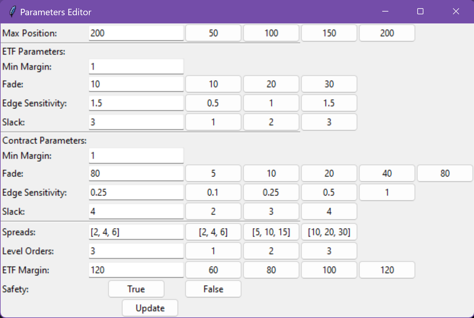
The blog post by Tianyi (Austin) Liu actually gave us many ideas to make our bots more robust, including the edge and fade parameters.Edge
Quoting from the blog post:It’s nice to be able to make a $.10 edge on each trade, but with 15 other market makers in the market, you won’t get to make any trades. So let’s reduce our edge to $.05. What happens in situations where there are no other market makers quoting in the market? Should you be satisfied with only $.05 in edge?Tianyi implements this edge by constantly checking and adjusting the edge of the bot. This is possible in his case, for there were only a single contract being traded. Unfortunately, it quickly appears to us that it is impossible to monitor 8 different assets and tune this parameters in real-time - we needed more robustness. Therefore, we specifically uses a tanh function to adjust the margins more aggressively towards either extremes of the margin range. We can then tune the parameters to adjust the aggressiveness of the autoadjustment. $$ \text{edge} = \text{int}(\text{round}(\text{min_margin} + (\frac{\text{slack}}{2} \times (\tanh(-4\times \text{edge_sensitivity} \times \text{activity_level} + 2)))))$$
Fade
Meanwhile, the fade parameter comes in handy when your positions are too imbalanced. For example, if you are holding 100 EPT, and this number keeps increasing, then it is very likely that your predicted price is too high (you are placing very favorable bids, but also very bad asks). Then, you might want to automatically adjust your prediction using the fade parameters. $$ \text{fade} = -f \times \text{sign}(\text{position}) \times \log_2(1 + \text{abs}(\text{position}))$$. Here \(f\) is the fade factor, which is a constant that we can tune to adjust the aggressiveness of the auto adjustment. I specifically used the \(\log\) function to heavily punish medium-sized imbalances (about half of the maximum position), so as we don't make premature adjustments, yet also do not delay the adjustment too much.GUI
Another enhancement inspired by Tianyi, yet we took a step further, is to create a GUI for our bots, which allows us to quickly monitor and tune the hyperparameters. We used x11 port forwarding, which allows us to run the GUI on the ssh server and display it on our screen. Apparently we won the (superlative) category of best GUI of the competition 😎